Einsum is All You Need
At the heart of every ML framework are matrix operations; ML related codebases are filled with (sometimes clever) matrix multiplications, transposes, and reductions. You can find einsum implementations in numpy, torch, and tensorflow, and you’ve probably seen it somewhere if you’ve looked at some ML codebase. It did take me a while to understand it, though, with a couple tries before I was able to use it for problems. And I’m probably not alone (there are a lot of SO posts about einsum). But once you do understand it, you can replace multi-line, multi-function tensor manipulations with einsum, which is straightforward to read and easier to think about and write in. You don’t have to do explicit transposes so that you can get the argument tensor dimensions lined up the correct way with each other or so that you can get the output tensor directly in the shape you want, without needing an additional manipulation. It’s also pretty annoying to keep in mind information about matrix operation functions (eg. order of arguments, the right transpositions to apply to input tensors). A non-exhaustive list can include calculating inner and outer products, matrix-matrix, and matrix-vector multiplications.
I’ve typically just used the library function (eg. torch.einsum) whenever I would need it but I was curious about how it was implemented, which is why I want to make my own (worse) version of einsum and explore some ideas for how the naive idea can be made more efficient. But before we think about that, its probably helpful to first understand how to use einsum.
NB: Einsum is not actually invented by Einstein. This notation actually came from the notation in the eponymous Ricci calculus. Einstein just borrowed it for General Relativity, which popularized it.
Dimensions, Axes, and Indices
It’s easy to mix these terms up (at least for me). So here’s what I mean by each term.
Dimensions: The total number of independent directions (degrees of freedom) in your data structure. For example, a scalar has 0 dimensions, a matrix has 2 dimensions, and an image (height x width x RGB) has 3 dimensions.
Axes: A way to refer to each “direction” or dimension by an integer label, usually starting at 0. For example, in a 2D array of shape (3, 4) axis 0 runs “down” the rows (length 3) and axis 1 runs “across” the columns (length 4).
Indices: A label used to identify elements on a given axis. For example, with a matrix you specify 2 indices to uniquely identify an element. The first index corresponds to axis 0 (row) and the second index corresponds to axis 1 (col).
The Rules of The Game
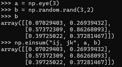
First let’s get familiar with the notation. If you’ve seen something like np.einsum("ij, jk -> ik", A, B) or np.einsum("ij, ik", A, B) (where A is some n X m matrix and B is some m X p matrix) before, you’ve already seen einsum :). This is a matrix multiplication where i and j are the labels associated with the axes of A. Similarly j and k are associated with the axes of B and i and k are the axes labels of the output. The repeating label (j in the above case) means that we multiply each row (since j is the second axis) of A with each column of B. In other words: whenever the same letter shows up in both array labels, einsum multiplies the matching entries along that axis and then sums over them.
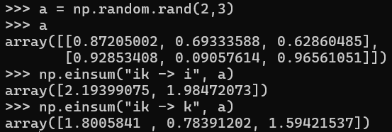
You can also do row or column reductions in einsum. np.einsum("ij -> i", A) sums the columns together for each row. This is done by omitting the column index j in the output. Similarly, the column reduction can be done using np.einsum("ij -> j"), where the rows for each column are summed together. In short: Omitting a letter from the output means that values along that axis will be summed.
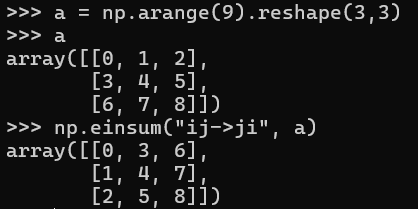
You might have noticed in the first example, you’d get the same output if the output axes were not explicitly specified. If you skip the -> and output labels, NumPy will automatically pick every index that appears only once, sort those letters alphabetically, and use them as the output. In other words, writing 'ij,jk->ik' is exactly the same as just 'ij,jk'. The benefit of specifying the output axes order is so we can transpose the output any way we like, by specifying the order of the argument (unsummed) axes in the output. An example transpose is shown below.
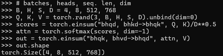
Einsum can be found in the wild in many different ways. For example, attention is able to elegantly be expressed with einsum:
A simple start
When you use einsum, you are probably thinking in terms of “contracting” axes (axes whose labels don’t appear in the output labels) and “free axes” (axes whose labels that do appear in the output labels). The contracted axes are axes whose dimensions are summed over (and optionally multiplied across if that axis labels appears more than once). For example with ij,jk->ik for two matrices A and B, i and k are free axes, while j is a contracted axis. A useful way to think of this is as a set of nested loops. You loop over all combinations of free axes (i,k) and sum the product A[i,j]*B[j,k]. Concretely:
A = torch.rand([2,3]) # [i,j]
B = torch.rand([3,4]) # [j, k]
result = torch.zeros([A.shape[0], B.shape[1]])
for i in range(A.shape[0]):
	for k in range(B.shape[1]):
		total = 0
		for j in range(A.shape[1]):
			total += A[i,j]*B[j,k]
		result[i,k] = total
If k was not specified as an output axis (so if we had ij,jk->i), then we’d just sum over the axis that is missing. So we’d have an intermediate matrix of ik, that we reduce over to get i by doing torch.sum(result, dim=missing_axes_indices). Here the missing_axes_indices=[1] since we’re reducing over k.
We can directly generalize this approach to work for any number of input and output axes. To make the initial implementation tractable, I made a couple of pretty significant restrictions on the functionality of this “barebones einsum”:
- Only take in two tensors
- Assume “common dimensions” are at the same position in both tensors
So it should be able to handle cases like:
ij, jk-> ikjilw, jekw-> ik(variable number of axes + sum reduce along appropriate axes)j, jkl-> k(different numbers of axes in each tensor) But not (yet) cases like:jilw, jekw-> ki(output axes appear in different order than input axes)ji, jk-> jik(duplicate axes)ij, i -> j(broadcasting)
What is broadcasting?
Broadcasting is the set of rules by which libraries like NumPy or PyTorch let you do element-wise operations on tensors of different shapes without writing explicit loops or reshaping every time. Under the hood, dimensions of size 1 (or missing trailing dimensions) are “stretched” (virtually, without extra memory) to match the other operand’s size. **Rules:** Compare the dimensions of two tensors from right to left. For each pair of dimensions `a_i` and `b_i`, they’re compatible if `a_i == b_i` or if one of them is 1. If they are, PyTorch/NumPy “stretches” the dimension of size 1 to match the other. The resulting dimension size is the maximum of the two.
Although this is a pretty nerfed version of einsum, we still need to:
- Implement einsum string parsing
- Reduce contracting axes
- Reduce axes that don’t appear in the output
The output of the parser allows us to generalize the above loop implementation to any number of free and contracting axes:
def barebones_einsum(tensor_a, tensor_b, common_dims, output_shape, reduce_dims):
    # Implementation of einsum without transposes

    # Assume common dims are at the same position in both tensors
    # common_dims_a, common_dims_b = common_dims, common_dims
    result = torch.zeros(output_shape)

    # Ranges for free (noncommon) dimensions (for iteration)
    a_noncommon_ranges = [range(size) for idx, size in enumerate(tensor_a.shape) if idx not in common_dims]
    b_noncommon_ranges = [range(size) for idx, size in enumerate(tensor_b.shape) if idx not in common_dims]

    # Cartesian products: all possible indices for non-common dims
    a_index_combinations = product(*a_noncommon_ranges)
    b_index_combinations = product(*b_noncommon_ranges)

    # Iterate over all combinations of non-contracted indices
    for a_indices, b_indices in product(a_index_combinations, b_index_combinations):
        common_index_ranges = product(*[range(tensor_a.shape[dim]) for dim in common_dims])
        total = 0
        for common_indices in common_index_ranges:
            # Build full indices including common dimensions
            full_a_indices = list(a_indices) # indices for non-common axes of A
            full_b_indices = list(b_indices) # indices for non-common axes of B

            for dim_idx, common_idx in enumerate(common_indices):
                # Insert cur common idx at the position of the dim in common_dims
                full_a_indices.insert(common_dims[dim_idx], common_idx)
                full_b_indices.insert(common_dims[dim_idx], common_idx)
            total += tensor_a[*full_a_indices] * tensor_b[*full_b_indices]

        # Store the total in the result tensor
        result[a_indices + b_indices] = total
    if len(reduce_dims) > 0:
        result = result.sum(reduce_dims)
    return result
This is essentially the same logic as the first set of loops we saw. Just now, we’ve expanded to handle more than matrix (2D) multiplications. This also supports broadcasting.
Inputs that work
# Tensor multiplication (no transposes)
tensor_a = torch.rand(3, 2, 4, 2)
tensor_b = torch.rand(3, 3, 5, 2)
example_str = "jilw, jekw-> ik"

# Broadcasting
tensor_a = torch.rand(3)
tensor_b = torch.rand(3, 2, 2)
example_str = "j, jkl-> k"
Details
Lets use the tensors a=torch.rand(2,1,1) and b=torch.rand(2,1,3) for the sake of an example. The common_dim, output_shape , and reduce_dim are:
common_dims=[0,1]
output_shape=torch.Size((1,3))
reduce_dims=[0]
This setup is equivalent to ijl, ijk -> k in einsum notation. We use the fact that the common dimensions in both tensors are specified using the same character and that we don’t specify a non-contracting (free) dimension l in the output to infer that l is reduced to get common_dims and reduce_dims .
It’s important to note that the output_shape is the shape before reductions. We contract over the common dims so before reduction we end up at something with shape (1,3) . After reducing the zeroth axis, we end up at something with shape (3,).
Python Unpacking
I’ll be using syntax like tensor[*indices], which unpacks the list of indices. This means that tensor_a[*[i, j, k]] is exactly the same as tensor_a[i, j, k].
We then use itertools.product to replicate and extend the outer two loops from the first example. This allows us to efficiently compress n loops if we have n free indices. for a_indices, b_indices in product(a_index_combinations, b_index_combinations): loops over all the free indices.
So for the example, we iterate over the following a_indices and b_indices which corresponds to the last axis for both A and B:
a_indices=(0,); b_indices=(0,)
a_indices=(0,); b_indices=(1,)
a_indices=(0,); b_indices=(2,)
Inside this loop, we have another loop which iterates over the common/contracting indices (again, we use itertools.product to cleanly handle multiple contracting dimensions. We sum over the contracting dimensions by slotting in contracting indices in their respective axes into both tensors (we assume same location of contracting axes in the input tensors). For the example, we multiply and sum elements in the following waytotal += tensor_a[*full_a_indices] * tensor_b[*full_b_indices]from A and B that are indexed in the following way (the first two axes are contracting axes in our example):
full_a_indices=[0, 0, 0]; full_b_indices=[0, 0, 0]
full_a_indices=[0, 1, 0]; full_b_indices=[0, 1, 0]
full_a_indices=[1, 0, 0]; full_b_indices=[1, 0, 0]
full_a_indices=[1, 1, 0]; full_b_indices=[1, 1, 0]
full_a_indices=[0, 0, 0]; full_b_indices=[0, 0, 1]
full_a_indices=[0, 1, 0]; full_b_indices=[0, 1, 1]
full_a_indices=[1, 0, 0]; full_b_indices=[1, 0, 1]
full_a_indices=[1, 1, 0]; full_b_indices=[1, 1, 1]
full_a_indices=[0, 0, 0]; full_b_indices=[0, 0, 2]
full_a_indices=[0, 1, 0]; full_b_indices=[0, 1, 2]
full_a_indices=[1, 0, 0]; full_b_indices=[1, 0, 2]
full_a_indices=[1, 1, 0]; full_b_indices=[1, 1, 2]
After summing the products for each element in the output (which is of shape (1,3) ), we then reduce the zeroth axis by summing over it with result.sum(reduce_dims) , which gives us the final shape of (3,) .
Building the Einsum Parser
It’s quite annoying to write out the reduce and common dims each time. We can easily infer this from the einsum string in the following way:
def parse_faster_einsum(einsum_str, tensors):
    if "->" in einsum_str:
        input, output = einsum_str.split("->")
        output_labels = list(output.strip())
    else:
        input = einsum_str
        output_labels = None

    input_labels = [list(op.strip()) for op in input.split(',')]
    assert len(input_labels) == len(tensors), "Number of inputs specified in str does not match number of tensors"
    return input_labels, output_labels
Given the input and output labels, we can infer the common dimensions (same character across tensors) and the reduce dimensions (free dimensions that don’t appear in the output labels).
Faster Einsum
Python loops are cool, but slow. This probably not a great thing to use when we want to use it for tasks that require many tensor operations. Luckily, GPUs/matmul kernels exist.

Some smart people have implemented super fast matrix multiplication kernels (that run on GPUs). Maybe we can use these kernels instead of python loops? We just need to reorder the axes and combine the axes so that we get matrices (rows and cols) from the input tensors. We can then replace the loops with a efficient matrix multiplication.
Structure
We can think of einsum as split into 3 stages after parsing. First, we get the intermediate output and intermediate labels. This is the result of the tensor multiplication (what we get after summing over the common dims). We then reduce along the relevant axes and permute the final axes so that we match the output axes order. We previously didn’t support transposes (where the output axes order was different than the free axes order). Now, keeping track of the intermediate labels we can support this. In code, this looks something like this:
# WARNING: The tensor updates are in-place. This might mean that tensors might be changed afterwards.
def faster_einsum(einsum_str, tensors):
    input_labels, output_labels = parse_faster_einsum(einsum_str, tensors)
    intermediate_tensor, intermediate_labels = einsum_pair(tensors[0], tensors[1], input_labels[0], input_labels[1], output_labels)

    # See if there are extra axes to reduce based on output shape
    sum_reduce_axes = [i for i, contract in enumerate(intermediate_labels) if contract not in output_labels]
    if len(sum_reduce_axes) > 0:
        for idx in sorted(sum_reduce_axes, reverse=True):
            del intermediate_labels[idx]
        result = intermediate_tensor.sum(dim=sum_reduce_axes)
    else:
        result = intermediate_tensor
    return result.permute(*[output_labels.index(label) for label in intermediate_labels])
Summing over Common Dims using Matrix Multiplication
The reason for trying to get to a matrix multiplication is so that we can use efficient GEMM kernels instead of for loops. The main idea is to separate the tensors into contracting and free axes and then reorder the axes of both tensors A and B in the following way:
A: [*free_axes_A, *contracting_axes]
B: [*contracting_axes, *free_axes_B]
We then flatten them to matrices (so that they have only 2 axes), which GEMM expects.
A: [math.prod(free_axes_A), math.prod(contracting_axes)]
B: [math.prod(contracting_axes), math.prod(free_axes_B)]
Since the contracting_axes list is the same for both A and B , we can guarantee that the matrix multiplication is going to be of form ij, jk -> ik.
Why does flattening and multiplying the resulting matrices give the same result as the tensor multiplication?
Let’s say we’re given two tensors `A` of shape $I \times J \times L$ and `B` of shape $I \times J \times K$, where $K$ and $L$ are the free dimensions. Normally we think of multiplying `A` and `B` as the following summation: $$ A^T@B = \sum_{i=0}^{I-1} \sum_{j=0}^{J-1} A_{i,j,\ell} \times B_{i,j,k} $$ The inner two loops can be combined into one by reshaping the matrices. If we combine the common dimensions such that `A` has shape $(i \times j) \times l$ and `B` has shape $(i \times j) \times k$, then we get an equivalent summation to the above in the following form: $$ \sum_{q=0}^{IJ-1} A_{\left\lfloor \tfrac{q}{J} \right\rfloor,\; q \bmod J,\; \ell} \times B_{\left\lfloor \tfrac{q}{J} \right\rfloor,\; q \bmod J,\; k} $$ We “flattened” our two contraction indices $(i,j)$ into one big index $q$ using the mapping $q = i \times J + j$ and the reverse mapping: $$ i = \left\lfloor \frac{q}{J} \right\rfloor, \quad j = q \bmod J. $$ Since we show both a forward and reverse mapping between our old indices and new index, we demonstrate that we cover each pair $(i,j)$ exactly once.
Given the input and output labels, we can infer the free and common dims/axes in the following way:
shared = set(labels_A) & set(labels_B)

contract_dims = [d for d in shared
           if (output_labels is None or d not in output_labels)]
free_A_dims = [d for d in labels_A
               if d not in contract_dims]
free_B_dims = [d for d in labels_B
               if d not in contract_dims]

free_axes_A = [labels_A.index(d) for d in free_A_dims]
contract_axes_A = [labels_A.index(d) for d in contract_dims]

contract_axes_B = [labels_B.index(d) for d in contract_dims]
free_axes_B = [labels_B.index(d) for d in free_B_dims]
We use the axes for keeping track of the labels (which we need later in the code for supporting transposed outputs). We use the dims to quickly calculate the respective products of the free and common axes. Torch takes care of broadcasting for us so we can just do the tensor manipulations explained above in code in the following way:
# Change axes order to allow (future) matrix multiplication (ie. [Free axes, Contract axes] @ [Contract axes, Free axes])
perm_A = A.permute(batch_axes_A + free_axes_A + contract_axes_A)
perm_B = B.permute(batch_axes_B + contract_axes_B + free_axes_B)

bA_shape = [perm_A.shape[i] for i in range(len(batch_axes_A))]
bB_shape = [perm_B.shape[i] for i in range(len(batch_axes_B))]

fA_shape = [perm_A.shape[len(batch_axes_A) + i] for i in range(len(free_axes_A))]
c_shape  = [perm_A.shape[len(batch_axes_A) + len(free_axes_A) + i] for i in range(len(contract_axes_A))]
fB_shape = [perm_B.shape[len(batch_axes_B) + len(contract_axes_B) + i] for i in range(len(free_axes_B))]

fA_prod = math.prod(fA_shape) if fA_shape else 1
c_prod  = math.prod(c_shape)  if c_shape  else 1
fB_prod = math.prod(fB_shape) if fB_shape else 1

A_mat = perm_A.reshape(*bA_shape, fA_prod, c_prod)   # (..., m, n)
B_mat = perm_B.reshape(*bB_shape, c_prod, fB_prod)   # (..., n, p)

C_mat = A_mat@B_mat
C = C_mat.reshape(*C_mat.shape[:-2], *fA_shape, *fB_shape)
C_labels = batch_dims + free_A_dims + free_B_dims
You might’ve noticed, that although we can now do transposes, this implementation is still restricted in the kinds of einsums we can do. For example, this still doesn’t support duplicate axes (like ji, jk-> jik) and more importantly, we’re still restricted to two inputs. We’re going to take care of these later but at least its faster, right?
Yes, How Much Faster?
We’re going to do a more thorough comparison later but for now here are the preliminary results for the following vanilla test case:
    tensor_a = torch.rand(3, 2, 4, 2)
    tensor_b = torch.rand(3, 3, 5, 2)
    example_str = "jilw, jekw-> ik"
We see that we’re much faster than the loops version. I also noticed that we’re a bit faster than the torch implementation of the full einsum. This is to be expected since we don’t handle a lot of cases that the torch version does.
| Implementation | Duration (seconds) |
|---|---|
| Torch | 2.01e-05 |
| Loops | 362.79e-05 |
| Matrix Mult. (Barebones) | 1.55e-05 |
Supporting More Than Two Inputs
We’ve only supported two tensor inputs so far. I wanted to solve the problem of tensor multiplication with two tensors first because we can use that logic to chain multiplications to support more than two tensors, since a contraction is just repeated sums of products:
\[\sum_{i,j,k,\dots} A_i\,B_j\,C_k\,\cdots\;=\;\sum_{k}\Bigl(\sum_{j}\bigl(\sum_{i}A_i\,B_j\bigr)\,C_k\Bigr)\,\cdots\]And since addition and multiplication are associative and commutative, we can group those sums in any **order. A simple one to start with is from left to right (where we keep a running product of the leftmost k elements). Concretely, left to right would look like:
- Do einsum(A,B)
- Then contract that result with C
- Then with D…
In code
We add a for loop going through tensors from left to right.
# WARNING: The tensor updates are in-place. This might mean that tensors might be changed afterwards.
def faster_einsum(einsum_str, tensors):
    input_labels, output_labels = parse_faster_einsum(einsum_str, tensors)
    # For now, we just go left to right
    left_tensor, intermediate_labels = tensors[0], input_labels[0]
    label_lists = input_labels[:]
    for i in range(1, len(tensors)):
        global_count = Counter(sum(label_lists, []))
        left_tensor, intermediate_labels = einsum_pair(
            left_tensor, tensors[i], intermediate_labels, input_labels[i], output_labels, global_count
        )
        label_lists = [intermediate_labels] + label_lists[2:]

    # See if there are extra axes to reduce based on output shape
    sum_reduce_axes = [i for i, contract in enumerate(intermediate_labels) if contract not in output_labels]
    if len(sum_reduce_axes) > 0:
        result = left_tensor.sum(dim=sum_reduce_axes)
    else:
        result = left_tensor
    # transpose to match the ordering specified in output_labels
    # eg. ikjr -> ikj -> jik
    for axis in sorted(sum_reduce_axes, reverse=True):
        del intermediate_labels[axis]
    return result.permute(*[output_labels.index(label) for label in intermediate_labels])
I chose left to right cause its the first thing that came to mind, but after thinking about it a bit longer, there is probably a better ordering. The order we pick these pairwise einsums probably affects the memory and compute needed. This is because we’d get a different chain of intermediate results (each with a different size). We could get big intermediate tensors, whose axes would later be summed over anyways. For example, lets say we have three tensors with the following shapes:
A: torch.Size((1000 x 10))
B: torch.Size((10 x 1000))
C: torch.Size((1000 x 10))
and we want to calculate the expression ab,bc,cd->ad . If we go left to right it would take the following memory and compute requirements.
- Contract
AandB:- Shapes: (1000,10) @ (10,1000) → (1000,1000)
- Cost: 1000*10*1000*2 = 2e7 FLOPS
- Two free dimensions of size 1000 and one common dimension of size 10. Each time we do two operations (an addition and a multiplication:
acc += A[i, k] * B[k, j])
- Two free dimensions of size 1000 and one common dimension of size 10. Each time we do two operations (an addition and a multiplication:
- Intermediate size: 1000*1000=1e6 elements
- Contract result with
C:- Shapes: (1000,1000) @ (1000,10) → (1000,10)
- Cost: 1000*1000*10*2 = 2e7 FLOPS
- Cost
- Compute: 4e7 FLOPs
- Peak memory: 1e6 elements
The optimal ordering would instead contract B and C first and then contract the result with A . This would use 4e7 FLOPS and have a peak memory usage of 100 elements, which is multiple orders of magnitude more efficient. In general to calculate the cost of a tensor multiplication, we multiply the sizes of the free dims of A with the sizes of B with the sizes of the common dimensions. Given this, we can just, at each step, pick the two tensors that would be the cheapest to compute. This would be more efficient that our naive left to right strategy most of the time, but still probably wouldn’t guarantee the most efficient ordering (since there may exist some orderings where you might need to take a more expensive intermediate tensor multiplications that will pay off for later multiplications).
This is how I implemented it
To find the best tensor pair, this requires a O(n**2) operation, but for most reasonable einsums n is small. We calculate the cost as described above.
def estimate_contraction_cost(tensor_A_shape, tensor_B_shape, labels_A, labels_B, output_labels, global_count):
    shared = set(labels_A) & set(labels_B)
    contract_dims = [d for d in shared
                    if global_count[d] == 2
                    and (output_labels is None or d not in output_labels)]
    batch_dims = [d for d in shared if d not in contract_dims]
    free_A_dims = [d for d in labels_A if d not in batch_dims and d not in contract_dims]
    free_B_dims = [d for d in labels_B if d not in batch_dims and d not in contract_dims]

    # Calculate output tensor size
    output_size = 1
    # Batch dimensions
    for d in batch_dims:
        idx_A = labels_A.index(d)
        idx_B = labels_B.index(d)
        output_size *= max(tensor_A_shape[idx_A], tensor_B_shape[idx_B])

    # Free dimensions from both tensors
    for d in free_A_dims:
        output_size *= tensor_A_shape[labels_A.index(d)]
    for d in free_B_dims:
        output_size *= tensor_B_shape[labels_B.index(d)]

    return output_size

def find_best_contraction_pair(tensors, label_lists, output_labels, global_count):
    min_cost = float('inf')
    best_pair = (0, 1)

    for i in range(len(tensors)):
        for j in range(i + 1, len(tensors)):
            cost = estimate_contraction_cost(
                tensors[i].shape, tensors[j].shape,
                label_lists[i], label_lists[j],
                output_labels, global_count
            )
            if cost < min_cost:
                min_cost = cost
                best_pair = (i, j)

    return best_pair

def faster_einsum(einsum_str, tensors, use_greedy=True):
    input_labels, output_labels = parse_faster_einsum(einsum_str, tensors)
    tensors = list(tensors)  # Make a copy so we can modify the list
    label_lists = input_labels[:]

    if not use_greedy:
        # Original left-to-right strategy
        left_tensor, intermediate_labels = tensors[0], input_labels[0]
        for i in range(1, len(tensors)):
            global_count = Counter(sum(label_lists, []))
            left_tensor, intermediate_labels = einsum_pair(
                left_tensor, tensors[i], intermediate_labels, input_labels[i], output_labels, global_count
            )
            label_lists = [intermediate_labels] + label_lists[2:]
    else:
        # Greedy strategy
        while len(tensors) > 1:
            global_count = Counter(sum(label_lists, []))
            i, j = find_best_contraction_pair(
                tensors, label_lists, output_labels, global_count
            )

            # Contract the chosen pair
            result, new_labels = einsum_pair(
                tensors[i], tensors[j], label_lists[i], label_lists[j], output_labels, global_count
            )

            # Remove the contracted tensors and their labels (larger index first)
            tensors.pop(max(i, j))
            tensors.pop(min(i, j))
            label_lists.pop(max(i, j))
            label_lists.pop(min(i, j))

            # Add the result back
            tensors.insert(0, result)
            label_lists.insert(0, new_labels)

        left_tensor = tensors[0]
        intermediate_labels = label_lists[0]
NB: I think (and don’t quote me on this) that torch uses this implementation instead, which is a dynamic programming approach.
Results
Let’s compare how fast our implementations are compared to torch’s version of einsum. I made some test cases of the scenarios which I thought were useful to test for. Here are their runtimes in seconds.
| Test Case | Einsum String | Tensor Shapes | PyTorch Time (s) | Left-to-Right Time (s) | Greedy Time (s) | Two Tensor/Matrix Mult. Time (s) | Barebones Time (s) |
|---|---|---|---|---|---|---|---|
| Greedy Optimization Case | ijk,kli,lm->ijm | A:(10,2000,30) B:(30,40,10) C:(40,50) | 6.67e-3 | 2.51e-3 | 5.14e-4 | N/A | N/A |
| Two inputs no transpose (broadcasting) | j, jkl-> k | A: (3). B: (3,2,2) | 1.48e-5 | 4.52e-5 | 2.24e-5 | 2.45e-5 | 2.87e-3 |
| Three inputs (simple) | ji, jk, jl -> ikl | A: (3,2) B: (3,3) C: (3,4) | 2.51e-5 | 5.81e-5 | 3.26e-5 | N/A | N/A |
| Two inputs duplicates | ji, jk-> jik | A: (3,3) B: (3,2) | 1.26e-5 | 2.21e-5 | 1.87e-5 | N/A | N/A |
| Two inputs | jilw, jekw-> ki | A: (3,2,4,2) B: (3,3,5,2) | 2.56e-5 | 4.10e-5 | 2.05e-5 | 1.82e-5 | N/A |
| Two inputs no transpose | jilw, jekw-> ik | A: (3,2,4,2) B: (3,3,5,2) | 1.93e-5 | 3.02e-5 | 2.15e-5 | 1.55e-5 | 3.92e-3 |
| Two inputs (broadcasting) | ij, i -> j | A: (3,2) B: (3) | 1.35e-5 | 1.50e-5 | 1.19e-5 | 8.42e-6 | N/A |
In the greedy optimization case, PyTorch’s default contraction path runs in 6.67 ms, while the naive left-to-right ordering completes in 2.51 ms. By contrast, the greedy heuristic finishes in just 0.71 ms, which is a 3.54× speedup over left-to-right! We also see that barebones is significantly slower than the other methods, which makes sense.
But these are just small inputs. Let’s see how they scale. We can scale in two ways: the tensor sizes and the number of tensors.
Runtime vs. Dimension Size
This table shows how each implementation scales with the size of each dimension (each dimension is the same size here so we have “square” tensors) with the einsum string ij,jk->ik. The runtimes are similar for all implementations. Interestingly, there seems to be a jump in runtime from when the size is 128 to when it is 256.
| Size | PyTorch (s) | Left-to-Right (s) | Greedy (s) |
|---|---|---|---|
| 4 | 1.5e-05 | 1.6e-05 | 1.3e-05 |
| 8 | 1.1e-05 | 1.6e-05 | 1.1e-05 |
| 16 | 1.2e-05 | 1.1e-05 | 1.3e-05 |
| 32 | 1.1e-05 | 1.1e-05 | 1.2e-05 |
| 64 | 1.1e-05 | 1.1e-05 | 1.3e-05 |
| 128 | 1.4e-05 | 1.4e-05 | 1.5e-05 |
| 256 | 3.5e-05 | 3.6e-05 | 3.4e-05 |
Runtime vs. Number of Tensors (square tensors)
This table shows how the runtime varies with the number of tensors. For this table each tensor is “square” with a size of 32. I use einsum strings that follow the chain multiplication pattern (ij,jk,kl,…). We see that left to right scales the best with square tensors. This makes sense as the other implementations have some extra overhead to optimize for when we have tensors with unequal dimension sizes. For example, with our greedy implementation we scale quadratically with the number of tensors (to find the best tensor pair to contract), while with left to right we don’t have this overhead.
Size = 32
| Num | PyTorch (s) | Left-to-Right (s) | Greedy (s) |
|---|---|---|---|
| 2 | 1.2e-05 | 1.0e-05 | 1.3e-05 |
| 3 | 2.0e-05 | 1.9e-05 | 2.5e-05 |
| 4 | 3.0e-05 | 2.9e-05 | 4.0e-05 |
| 5 | 4.4e-05 | 3.7e-05 | 5.6e-05 |
| 6 | 5.7e-05 | 4.6e-05 | 7.7e-05 |
Size = 8
| Num | PyTorch (s) | Left-to-Right (s) | Greedy (s) |
|---|---|---|---|
| 2 | 9.0e-06 | 8.0e-06 | 9.0e-06 |
| 3 | 1.6e-05 | 1.5e-05 | 1.8e-05 |
| 4 | 2.2e-05 | 2.1e-05 | 2.7e-05 |
| 5 | 3.4e-05 | 2.6e-05 | 4.0e-05 |
| 6 | 4.3e-05 | 3.2e-05 | 5.7e-05 |
Size = 16
| Num | PyTorch (s) | Left-to-Right (s) | Greedy (s) |
|---|---|---|---|
| 2 | 1.2e-05 | 1.3e-05 | 1.5e-05 |
| 3 | 2.1e-05 | 2.0e-05 | 2.7e-05 |
| 4 | 3.0e-05 | 2.9e-05 | 3.9e-05 |
| 5 | 5.8e-05 | 5.1e-05 | 7.3e-05 |
| 6 | 5.9e-05 | 4.6e-05 | 7.8e-05 |
Runtime vs. Unequal Tensor Dimensions
The optimizations we did for the contraction order were for the cases when the dimensions were varied (ie. when tensors were not squares). This table shows how the runtime varies with various orders of dimension sizes (for three tensors). We can see that for wide tensors with one small dim (the case when the outer dimensions for the first two tensors is large), we see an order of magnitude improvement of our greedy implementation compare to the left to right and torch ’s implementation (surprisingly).
| Case | PyTorch (s) | Left-to-Right (s) | Greedy (s) | Dimension Order |
|---|---|---|---|---|
| Very thin tensors with one large dim | 1.8e-05 | 1.8e-05 | 2.0e-05 | (2,1024) * (1024,2) * (2,1024) |
| Very wide tensors with one small dim | 3.5e-04 | 3.3e-04 | 3.8e-05 | (1024,2) * (2,1024) * (1024,2) |
| Small to large progression | 5.3e-05 | 5.2e-05 | 5.4e-05 | (2,2) * (2,1024) * (1024,1024) |
| Large to small progression | 1.2e-04 | 1.3e-04 | 1.3e-04 | (1024,1024) * (1024,2) * (2,2) |
| Diamond shape (small–large–large–small) | 3.3e-05 | 3.0e-05 | 3.3e-05 | (2,512) * (512,512) * (512,2) |
| Hourglass shape (large–small–small–large) | 5.0e-05 | 4.6e-05 | 3.8e-05 | (512,2) * (2,2) * (2,512) |
The pretty thing about einsum is that you don’t need to know how it works to use it. But implementing it myself has made me appreciate it more now. I started with nested Python loops to explicitly build index combinations, insert contracting axes, and summing over them. By “matricizing” tensors into [free, contract] @ [contract, free] and leaning on BLAS, a single batched matrix multiplication replaces those loops with years of low-level optimization. Along the way, I discovered that how you chain pairwise contractions matters just as much as what you contract. A fixed left to right schedule is easy to understand, but on unequal dimensions a simple greedy search for the cheapest next GEMM can slash both FLOPs and peak memory by orders of magnitude. On more balanced tensors, though, that search overhead can outweigh its own benefits (so sometimes a “dumber” strategy is actually smarter).