Building a Lego Set Identifier
With a bucket of Lego, you can tell any story. - Christopher Miller
We’ve all played with Lego, at one point or another, clicking together bricks to create whats on the box it came in or something entirely our own. But beyond childhood memories, there exists a massive, thriving second-hand Lego ecosystem that I was unaware existed. Here, people often buy and sell their Lego bricks once they’ve had their fun building whatever set each piece came from. There even exist brick and mortar stores where people show up with tubs of old Lego parts. Although more often its sold online on platforms like Bricklink, which see an absurd number of Lego pieces being traded every day.
Of course, with scale comes complexity. These second hand stores have actual humans sorting through these Lego buckets, a piece at a time. These pieces are often sold individually or in bulk, depending on how rare they are. However, sometimes they are also sold in sets, which yield a much higher average price per piece. But these second hand sets are time consuming to create (since they need to go around and collect the buckets of sorted pieces) and which set to create (based on their inventory) to maximize value. Other “bundles” are also sold, like incomplete sets and minifigures, but these tend to yield, on average, a lower average price per piece.
I got introduced to this ecosystem and problem through my friend’s startup. Right now, this sorting process is very much human based (and humans are expensive and they also make mistakes, making them non-ideal for tasks like these). His startup is building a machine to sort Lego pieces into individual buckets based on piece attributes like color or shape etc. However, unlike humans, machines can also directly sort pieces into sets, since they can remember how many of each piece every possible set has instead of first sorting to intermediate buckets by color or piece type. And maybe they can use this to figure out which bucket/set to sort this piece into to have the highest likelihood of getting a full, complete set at the end of sorting.
Incorporating some algorithm that optimally assigns each piece to each set directly would increase the average price per piece of the pieces sold, while allowing humans to focus on tasks they are better suited to. This task also seems interesting from a technical perspective. The task into is essentially a probabilistic, online optimization problem. The full contents of the tub are unknown, so the system must constantly update its belief about which sets are present. With each piece, it must decide on the fly where to assign it to maximize value. And exhaustively checking all combinations is intractable, so the problem calls for some approximation algorithms or sampling methods. Add real-world constraints like limited buckets, uncertain piece recognition, and noisy inputs, and you’ve got a genuinely rich AI problem blending vision, probabilistic reasoning, and decision-making under uncertainty.
Sidenote
This area seems to be a goldmine of interesting optimization problems. For example, we only have a fixed number of buckets we are sorting to, and we’re only going through the pieces once. Would it make more sense to do some sort of hierarchical sorting with multiple passes to optimize price per piece (where we’d have a better prior of pieces than using the initial unsorted buckets)? Another problem that is not discussed here would be optimizing not only for full, complete sets, but also for set value. So there’d be cases where we’d accept a lower likelihood of a full set if that set can be sold at a higher price.
Overview
We solve a simpler problem here to gain some traction to hopefully build up to some final version that can actually be used one day. We can frame this simpler problem as such:
Lego pieces are fed one by one from an unsorted bucket, which contains pieces from a mixture of Lego pieces. We have no prior knowledge of the distribution of pieces from buckets, so we have to make the best decision based on the pieces seen so far.
The problem is simpler through the assumption of the following limiting assumptions:
- Each set can only occur once
- The bucket is a mixture of N complete sets
- A generic prior (as opposed to a more informed prior which can be based on actual Lego statistics about number of sets produced in some region). We assume the bucket contains uniformly random sets.
We can define the problem as follows:
- $M$: Number of sets
- $S_j$: Lego set j
- $\pi_j$: The unknown proportion of set j in the bucket; $\sum_{j=1}^{M} \pi_j = 1$
Where the set-piece probability is defined as: $P(piece_k|S_j) = \frac{\text{count of piece}_k \text{ in set } S_j}{\text{number of pieces in set } S_j}$ We get this information using the Bricklink API.
We can also calculate the probability of seeing some piece from the unsorted bucket by:
\[P(\text{piece}_k \mid \pi) = \sum_{j=1}^{M} P(\text{piece}_k \mid S_j) \cdot P(S_j) = \sum_{j=1}^{M} P(\text{piece}_k \mid S_j) \cdot P(\pi_j)\]We want to calculate the posterior distribution using Bayes’ rule:
\[P(\pi \mid \text{observations}) \propto \underbrace{P(\text{observations} \mid \pi)}_{\text{likelihood}} \cdot \underbrace{P(\pi)}_{\text{prior}}\]We assume the prior to be a uniform distribution, where each set is equally likely.
The likelihood term can be re-written as:
where $n$ is the number of observations.
This would be easy enough to solve if we knew $\pi_j$, but we don’t :(.
I tried several approaches to estimate $\pi_j$, including Expectation Maximization and some MCMC methods. I compared the evaluated methods across different numbers of sets in the bucket, number of pieces seen, time taken to produce predictions, number of possible sets to choose from, and number of iterations. You can find the simulation and evaluation code here.
Expectation Maximization Math
This is the first algorithm that came to mind and we can use it out of the box for this problem. Its used to determine the maximum likelihood estimates of parameters when some of the data is missing. We’re trying to estimate the latent parameters (the unknown set assignments for each piece) [$\pi_1, \pi_2, …, \pi_n$] with incomplete data, [$piece_1, piece_2, …, piece_n$] (we don’t know the set identity of each observed piece). The EM process consists of iteratively applying two steps, the E(xpectation)-step and the M(aximization)-step, until we converge to some estimate of $\pi$ that maximizes the likelihood of the observed pieces.
E-Step
In this step, we compute the posterior probability that $\text{piece}_k$ came from set $S_j$, that is, $P(S_j \mid \text{piece}_k, \pi)$. Using Bayes’ rule, this can be written as:
\[\gamma_{kj} := P(S_j \mid \text{piece}_k, \pi) = \frac{P(\text{piece}_k \mid S_j) \cdot P(S_j)}{P(\text{piece}_k \mid \pi)} = \frac{P(\text{piece}_k \mid S_j) \cdot \pi_j} {\sum_{l=1}^{M} \pi_l \cdot P(\text{piece}_k \mid S_l)}\]Here, $\gamma_{kj}$ is a soft assignment of piece $k$ to set $S_j$.
M-Step
In this step, we update the estimates of $\pi_j$ based on the soft assignments calculated in the E-step. We just average over how much each piece belongs to each set: $\pi_j = \frac{1}{n}\sum_{k=1}^{n}\gamma_{kj}$
We stop iterating once no $\pi_j^{t+1}$ is more than some $\epsilon$ away to $\pi_j^{t}$.
MCMC Methods
Monte Carlo Markov Chain methods are a class of methods that allow us to approximate some characteristics about the population (like the mixture of sets in the bucket) by allowing easy sampling from a probability distribution (based on the pieces seen so far).
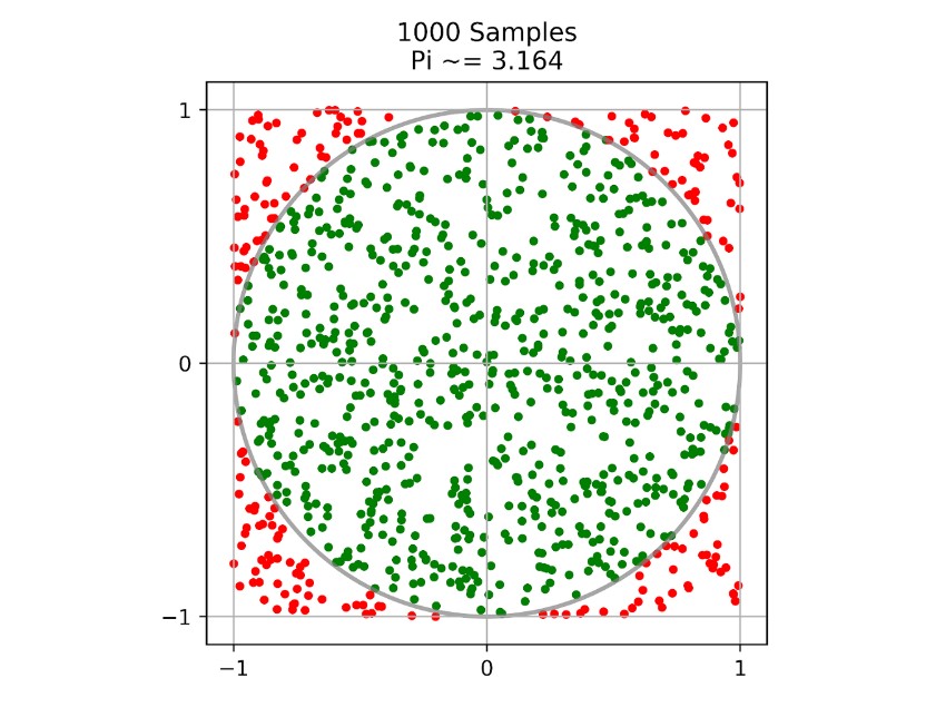
The monte carlo part of the MCMC refers to method of performing a simulation to approximate a quantity that would otherwise be hard to determine. For example you can use monte carlo sampling to approximate the area of a circle by randomly drawing points and seeing how many fall inside the circle.
However, sometimes—like in our case—it is hard to even sample points from a probability distribution.
As a reminder, we’re trying to determine $P(\pi \mid \text{observations})$ using the likelihood $P(\text{observations} \mid \pi)$.
The likelihood is given by:
This expression is difficult to sample from directly, due to the nested summation inside the product.
We can use Markov Chains (if you want an even more detailed understanding) to sample from an intractable probability distribution. These are useful, because these Markov Chains, after an initial burn in period, have a stationary distribution (over the states visited during the walk). If we can construct a Markov Chain such that this stationary distribution is the one we want to sample from, we have a way to efficiently sample from our probability distribution. Methods such as Metropolis Hastings or Gibbs Sampling construct some (implicit) Markov Chain such that this property holds.
Metropolis Hastings
At a high level, Metropolis Hastings works by running the following for a fixed number of iterations:
- Propose a new $\pi’$ near the current parameters value $\pi$. This is done using another distribution. I calculated $\pi’$ by adding $\pi$ to $x \sim \mathcal{N}(0, \epsilon)$, where $\epsilon$ is some hyperparameter.
- Accept or reject the proposed $\pi’$ with a probability that ensures that we eventually sample from the true posterior distribution, $P(\pi|observations)$. This acceptance probability turns out to be $\alpha = \min\left(1, \frac{P(\pi’ \mid \text{observations})}{P(\pi \mid \text{observations})}\right)$. Why this leads to a Markov Chain with a stationary distribution of our posterior is quite interesting. I used an exponential prior, where $P(\pi) = \prod_{j=1}^{M}exp(-\lambda\theta_j)$, to encourage sparsity (that few probabilities are far away from zero), which assumes that only a few sets relative to all the sets are in the bucket.
To avoid numerical instability (since we’d be dealing with pretty small floats) and simplify computations, I evaluated the log of the posterior instead of the posterior directly (exponential prior gets simplified and the acceptance ratio is now a difference). I still sample from the posterior, but use log-probabilities in the acceptance ratio to make the algorithm more stable and efficient.
log_accept_ratio = proposed_log_posterior - current_log_posterior
accept_ratio = np.exp(min(0, log_accept_ratio))
One downside of what I’ve done so far is that performance is dependent on the acceptance ratio. If the acceptance ratio is too low, then we’re failing to explore the space effectively. If it’s too high, then the sampled values are not varied and representative of the long tails of the distribution. Usually the target acceptance rate should be between 0.2 and 0.5. Since the acceptance rate depends on the $\epsilon$, I implement some logic to adapt $\epsilon$ to get an acceptance rate in the ideal range.
if sum_accept_ratios/len_accept_ratios < 0.2:
	eps *= 0.9 # reduce step size, increase acceptance rate
elif sum_accept_ratios/len_accept_ratios > 0.5:
	eps *= 1.1 # increase step size, reduce acceptance rate
...
sample_theta = theta + np.random.normal(0, eps, size=theta.shape)
Gibbs Sampling
Gibbs sampling is another MCMC method, which at a closer glance is really a special case of MH with an acceptance ratio of 1. Lets first see what Gibbs sampling is and then see how its basically a simpler version of MH.
Gibbs sampling allows us to sample from a joint distribution over multiple variables by breaking it into conditional distributions and sampling each variable conditioned on the latest value of all the other variables.
It consists of 2 steps:
- Randomly initialize set proportions $\pi^{(0)}$ and piece assignments $z_i^{(0)}$ for each observed piece i.
- Cycle through each parameter to calculate $P(\pi \mid \text{observations})$.
Here, we first sample which set each piece came from, given the mixture proportions. This is the Gibbs step for $z_i$. Then we perform the Gibbs step for $\pi$ by sampling a new $\pi$ based on the current set assignment counts (i.e., we calculate $P(\pi \mid z_1, \dots, z_n)$).
I modelled the distributions of $\pi$ using a Dirichlet distribution (since its conjugate with the categorial distribution). This means that since my prior is a Dirichlet distribution and my observations (set assignments) come from a categorical distribution, the posterior is also Dirichlet. $\pi∼\text{Dirichlet}(α_1,…,α_M)$ , with the $\alpha_j$ acting as a prior belief in how common set $j$ is before seeing the observations. The posterior also turns out to be Dirichlet because the prior is $P(\pi) = Dir(\alpha_1, …, \alpha_M) \propto \prod_{j=1}^{M}\pi_j^{\alpha_j-1}$ and the likelihood is $P(z|\pi) = \prod_{j=1}^{M}\pi_j^{n_j}$, where $n_j$ is the number of times the observed pieces were assigned to set $j$. Using Bayes’ rule, $P(\pi|z) = P(z|\pi)*P(\pi) \propto \prod_{j=1}^{M}\pi_j^{\alpha_j-1} * \prod_{j=1}^{M}\pi_j^{n_j} = \prod_{j=1}^{M}\pi_j^{\alpha+n_j+-1}$. This is the form of a Dirichlet distribution: $\pi|z ∼ Dir(\alpha_1+n_1, …, \alpha_M+n_M)$.
This approach models the latent structure (the piece assignments) explicitly, which maybe mixes faster than directly sampling over $\pi$? This is something I want to test during the experiments.
Experiments + Analysis
To evaluate the effectiveness of different inference strategies, I compared MH, adaptive MH, Gibbs Sampling, and EM across a wide range of settings.
Each method was tested on synthetic Lego buckets, where each bucket contains a mixture of Lego sets. The goal for each algorithm is to infer the most likely underlying set proportions based on observed pieces.
I pulled ~10,000 real Lego sets and their piece distributions at random using the Bricklink API, allowing us to use realistic piece distributions.
For each method, I varied the following four factors:
- Number of sets in the bucket:
ks = [1, 10, 100] - Number of pieces observed:
num_pieces = [10, 100, 1000] - Number of candidate sets to choose from:
num_sets_to_choose_from = [1000, -1](-1 means using the full ~10,000-set pool) - Number of iterations:
num_iterations = [1_000, 10_000, 100_000](for EM, this is capped rather than run to convergence)
Below are the plots that show the effect of each factor independently (all other factors are averaged over):
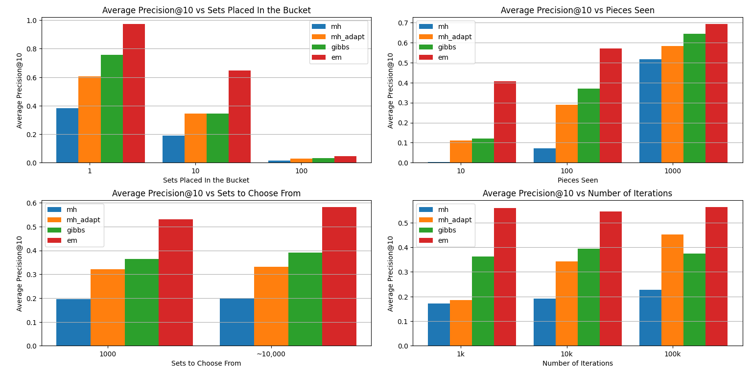 Performance drops sharply as more sets are added to the bucket. This is expected: with more sets present, the piece distribution becomes increasingly entangled and ambiguous, making it harder to attribute any single piece to the correct set, since every unique set of pieces that each set brings to the bucket, increases the potential sets the bucket could’ve come from. Interestingly, EM and Gibbs sampling outperform both versions of MH in this setting, especially when only one or ten sets are involved. MH struggles the most here, suggesting that it doesn’t explore the space well when the signal is faint and the posterior is highly multimodal. All methods consistently improve as more pieces are observed, which is makes sense: more evidence leads to better inference. However, vanilla MH shows the steepest curve, jumping from nearly useless at 10 pieces to decent performance at 100–1000. This suggests that MH may require a critical mass of observations to begin converging on useful hypotheses. In contrast, EM performs quite well even with very little data, which is surprising given its typical reliance on smooth likelihood surfaces.
As we increase the number of iterations, all methods improve which is not surprising; There are differences though:
- MH-adapt benefits the most from additional iterations, outperforming vanilla MH significantly at 100k steps.
- EM, surprisingly, performs quite well even with few iterations, suggesting that it reaches reasonable estimates quickly, even without full convergence.
- Gibbs performs consistently well, but doesn’t show as sharp a gain with more iterations, possibly due to the burn-in period being short relative to the total run.
Future work
I was surprised that EM showed such dominant performance over all tested factors. I honestly expected some methods, like MH-adapt to outperform EM when we had more iterations, but this doesn’t seem to be the case (for the tested values). Maybe an interesting path to explore in the future, could be to use 1000 iteration EM to set good priors for the MCMC methods, which can allow them to converge to more accurate predictions.
All current experiments use a uniform prior over sets. In the real world, some sets are far more common than others. Incorporating realistic prior distributions based on historical Lego production or second-hand market data from Bricklink, or even past classifications from the second hand Lego store could significantly improve early-stage predictions by setting better initializations. For example for EM, we use a uniform initialization, which is probably not true (this prior essentially says that each set is equally likely to be in the bucket). Also, the algorithms we looked at only try to reconstruct full sets. But some sets (e.g. rare or collectible ones) are much more valuable than others. Future models could factor in expected resale value, optimizing not just for reconstruction likelihood, but also for price per piece.
But I think we’ll use EM for now since this probably won’t become the bottle neck from a business perspective until much later.
Leg Godt :)